#01 | Getting Started with Pandas
A clear introduction to Pandas, a Python library to manipulate tabular data, where you can discover its many possibilities and get a concise overview.
Read the original article here, in Hashnode.
An array is any type of object that can store more than one object. For example, the list:
[100, 134, 87, 99]
Let's say we are talking about the revenue our e-commerce has had over the last 4 months:
list_revenue = [100, 134, 87, 99]
We want to calculate the total revenue (i.e., we sum up the objects within the list):
list_revenue.sum()
--------------------------------------------------------------------------- AttributeError Traceback (most recent call last) Input In [3], in <cell line: 1>()
----> 1 list_revenue.sum() AttributeError: 'list' object has no attribute 'sum'
The list is a poor object which doesn't contain powerful functions.
What can we do then?
We convert the list to a powerful object such as the Series, which comes from pandas library.
import pandas

pandas.Series(list_revenue)
>>>
0 100
1 134
2 87
3 99
dtype: int64
series_revenue = pandas.Series(list_revenue)
Now we have a powerful object that can perform the .sum():
series_revenue.sum()
>>> 420
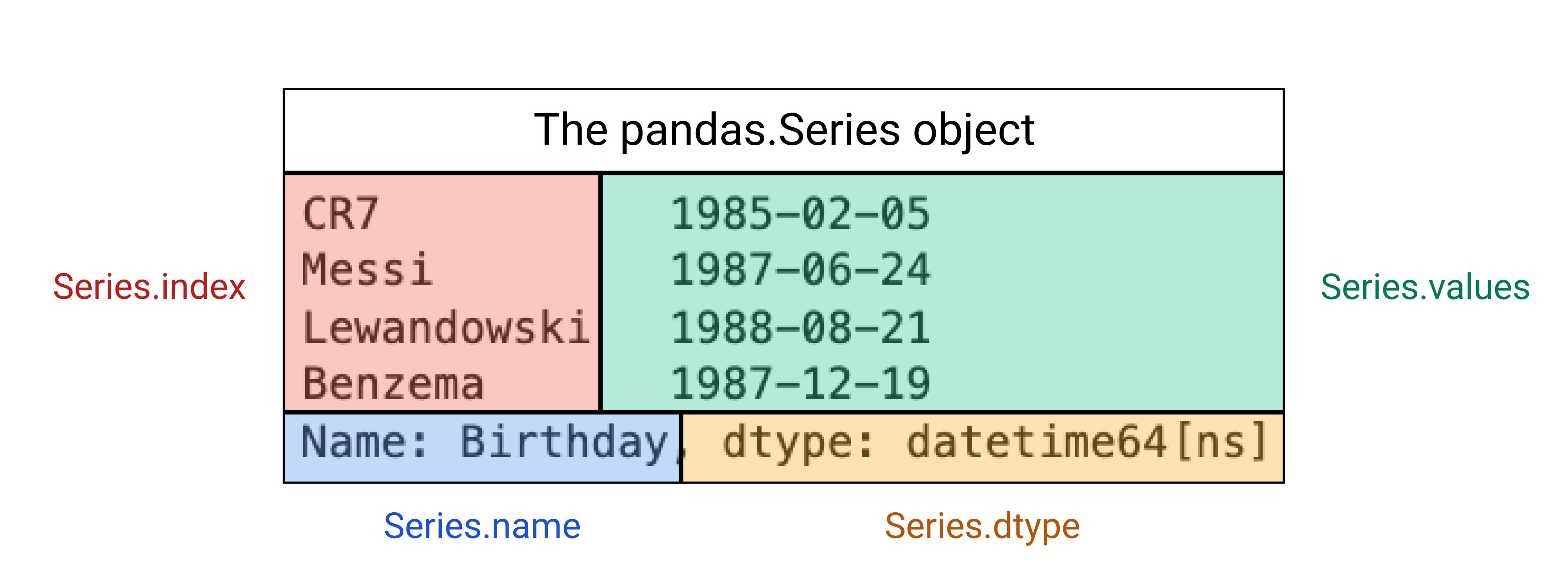
Within the Series, we can find more objects.
series_revenue
>>>
0 100
1 134
2 87
3 99
dtype: int64
series_revenue.index
>>> RangeIndex(start=0, stop=4, step=1)
Let's change the elements of the index:
series_revenue.index = ['1st Month', '2nd Month', '3rd Month', '4th Month']
series_revenue
>>>
1st Month 100
2nd Month 134
3rd Month 87
4th Month 99
dtype: int64
series_revenue.values
>>> array([100, 134, 87, 99])
series_revenue.name
The Series doesn't contain a name. Let's define it:
series_revenue.name = 'Revenue'
series_revenue
>>>
1st Month 100
2nd Month 134
3rd Month 87
4th Month 99
Name: Revenue, dtype: int64
The values of the Series (right-hand side) are determined by their data type (alias dtype):
series_revenue.dtype
>>> dtype('float64')
Let's change the values' dtype to be float (decimal numbers)
series_revenue.astype(float)
>>>
1st Month 100.0
2nd Month 134.0
3rd Month 87.0
4th Month 99.0
Name: Revenue, dtype: float64
series_revenue = series_revenue.astype(float)
What else could we do with the Series object?
series_revenue.describe()
>>>
count 4.000000
mean 105.000000
std 20.215506
min 87.000000
25% 96.000000
50% 99.500000
75% 108.500000
max 134.000000
Name: Revenue, dtype: float64
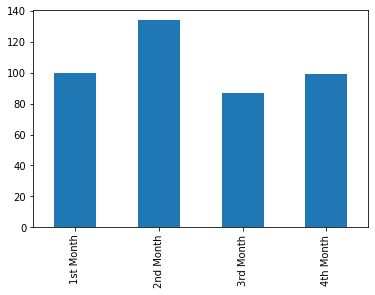
series_revenue.plot.bar();
series_revenue.plot.barh();

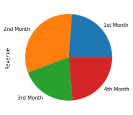
series_revenue.plot.pie();
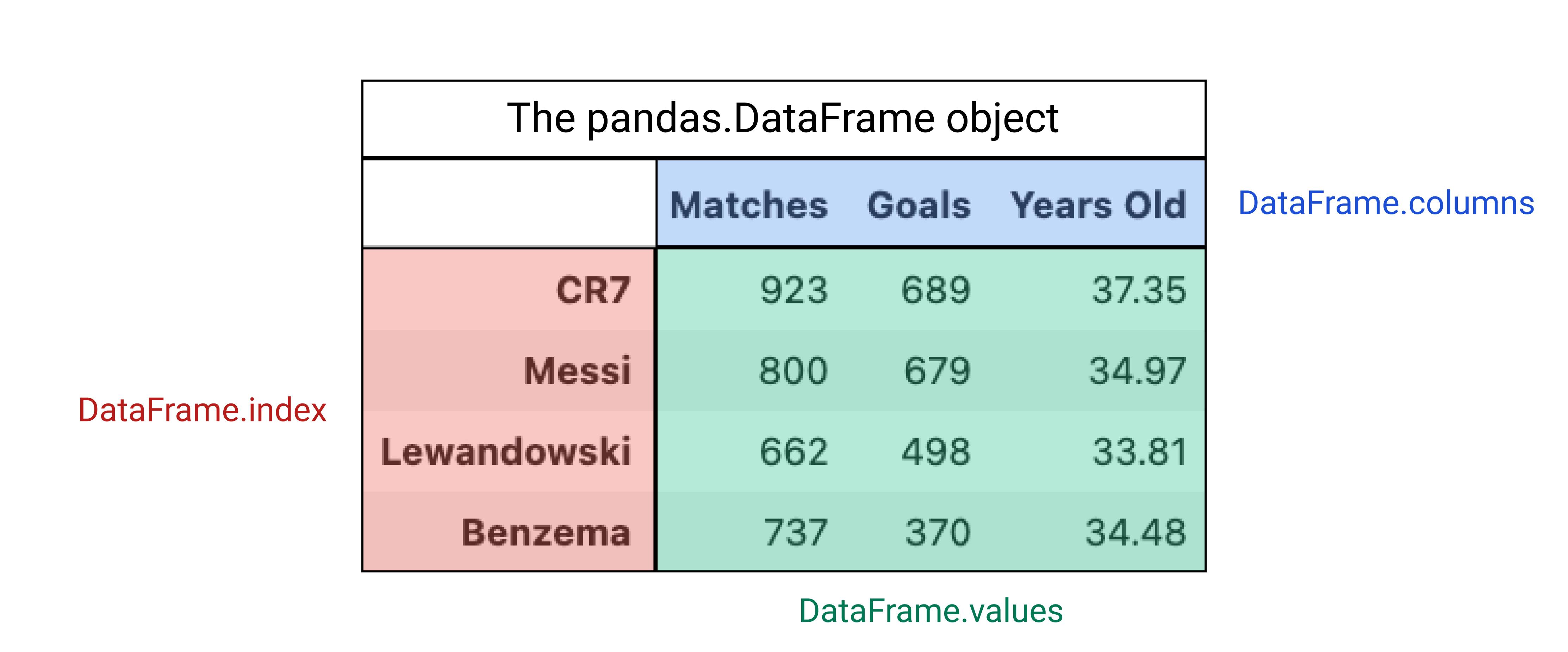
The DataFrame is a set of Series.
We will create another Series series_expenses to later put them together into a DataFrame.
pandas.Series( data=[20, 23, 21, 18], index=['1st Month','2nd Month','3rd Month','4th Month'], name='Expenses'
)
>>>
1st Month 20
2nd Month 23
3rd Month 21
4th Month 18
Name: Expenses, dtype: int64
series_expenses = pandas.Series( data=[20, 23, 21, 18], index=['1st Month','2nd Month','3rd Month','4th Month'], name='Expenses'
)
pandas.DataFrame(data=[series_revenue, series_expenses])

df_shop = pandas.DataFrame(data=[series_revenue, series_expenses])
Let's transpose the DataFrame to have the variables in columns:
df_shop.transpose()
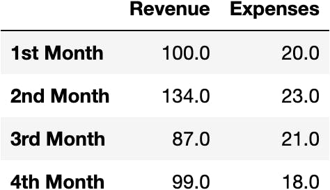
df_shop = df_shop.transpose()
df_shop.index
>>> Index(['1st Month', '2nd Month', '3rd Month', '4th Month'], dtype='object')
df_shop.columns
>>> Index(['Revenue', 'Expenses'], dtype='object')
df_shop.values
>>>
array([[100., 20.], [134., 23.], [87., 21.], [99., 18.]])
df_shop.shape
>>> (4, 2)
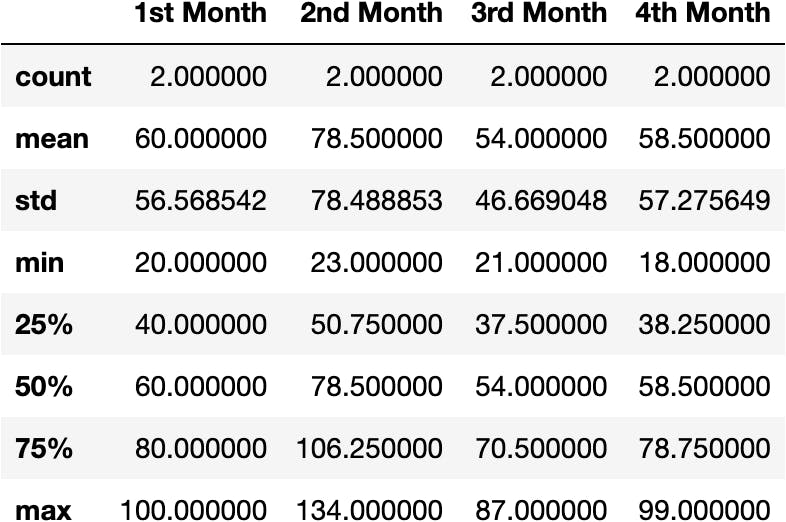
What else could we do with the DataFrame object?
df_shop.describe()
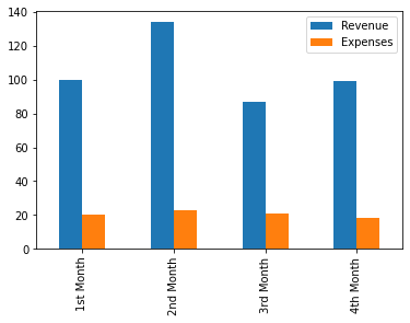
df_shop.plot.bar();
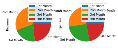
df_shop.plot.pie(subplots=True);
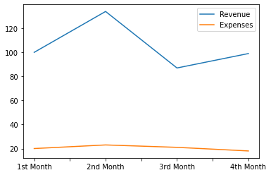
df_shop.plot.line();
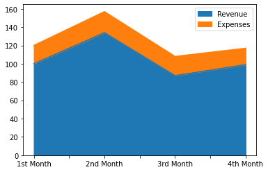
df_shop.plot.area();
We could also export the DataFrame to formatted data files:
df_shop.to_excel('data.xlsx')
df_shop.to_csv('data.csv')
url = 'https://raw.githubusercontent.com/jsulopzs/data/main/football_players_stats.json'
pandas.read_json(url, orient='index')

df_football = pandas.read_json(url, orient='index')
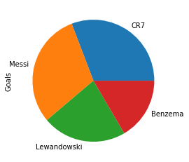
df_football.Goals.plot.pie();
url = 'https://raw.githubusercontent.com/jsulopzs/data/main/best_tennis_players_stats.json'
pandas.read_json(path_or_buf=url, orient='index')

df_tennis = pandas.read_json(path_or_buf=url, orient='index')
df_tennis.style.background_gradient()

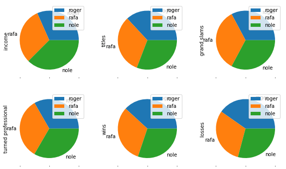
df_tennis.plot.pie(subplots=True, layout=(2,3), figsize=(10,6));
HTML Web Page
pandas.read_html('https://www.skysports.com/la-liga-table/2021', index_col='Team')[0]
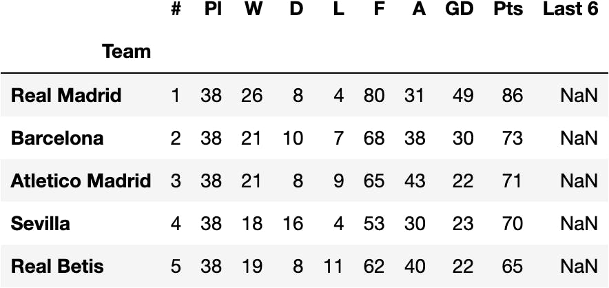
df_laliga = pandas.read_html('https://www.skysports.com/la-liga-table/2021', index_col='Team')[0]
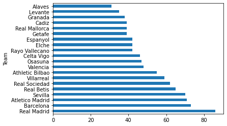
df_laliga.Pts.plot.barh();
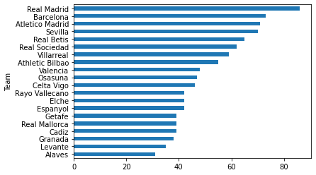
df_laliga.Pts.sort_values().plot.barh();
url = 'https://raw.githubusercontent.com/jsulopzs/data/main/internet_usage_spain.csv'
pandas.read_csv(filepath_or_buffer=url)
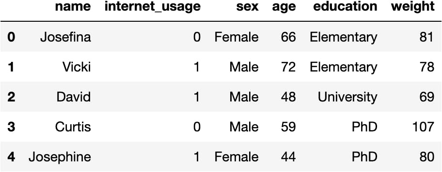
df_internet = pandas.read_csv(filepath_or_buffer=url)
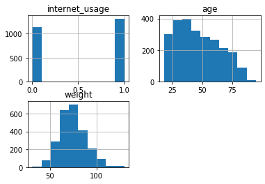
df_internet.hist();
df_internet.pivot_table(index='education', columns='internet_usage', aggfunc='size')
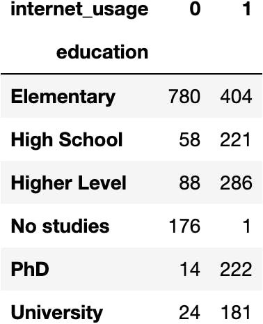
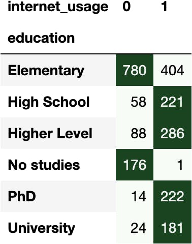
dfres = df_internet.pivot_table(index='education', columns='internet_usage', aggfunc='size')
dfres.style.background_gradient('Greens', axis=1)

This work is licensed under a Creative Commons Attribution-NonCommercial-NoDerivatives 4.0 International License.
